41 excel pivot table 2 row labels

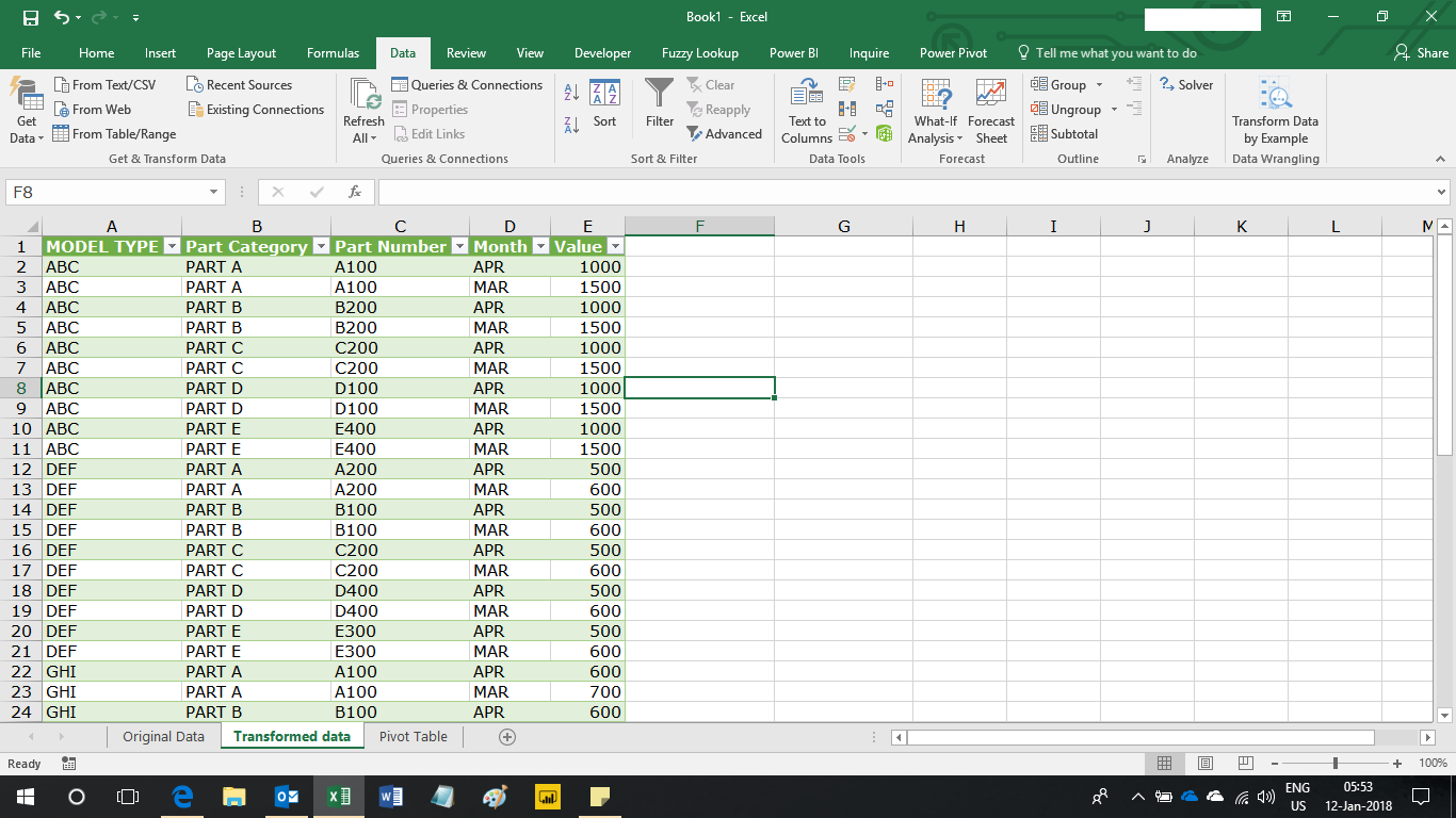
Combining two+ Columns to form one Row label column in Pivot Table Hello, I have multiple sets of data that occur in 2 column increments. The first column is a list of part numbers, the second is their value for that month. I want a pivot table that combines all of the first columns into one master row label of Part numbers and then the values will be listed out in each subsequent column. If a particular month doesn't have a part number in its data, then it ... Multiple row labels on one row in Pivot table | MrExcel Message Board I figured it out - Right click on your pivot table and choose pivot table options/display. Click on "Classic PivotTable layout" Then click on where it is subtotaling your row label and uncheck the subtotal option. D dudeshane0 New Member Joined Oct 23, 2014 Messages 1 Jan 19, 2015 #6 Gerald Higgins said:

Pivot Table Row Labels In the Same Line - Beat Excel! First make a pivot table with required fields. Arrange the fields as shown in left picture. Your initial table will look like right picture. Now click on "Error Code" and access field settings. First check "None" option in "Subtotals & Filters" tab to disable totals after every row.

Excel pivot table 2 row labels

get a row label from pivot table - Microsoft Tech Community @omdl2020 . GETPIVOTDATA() doesn't work in such case, it provides data if only it is visible in PivotTable. Alternatively you may work with cube assuming you are at least on Excel 2010, as I remember it's the first which supports data model. Remove PivotTable Duplicate Row Labels - Excel Help Forum Re: Remove PivotTable Duplicate Row Labels. Sometimes when the cells are stored in different formats within the same column in the raw data, they get duplicated. Also, if there is space/s at the beginning or at the end of these fields, when you filter them out they look the same, however, when you plot a Pivot Table, they appear as separate ... Pivot table row labels side by side - Excel Tutorials You can copy the following table and paste it into your worksheet as Match Destination Formatting. Now, let's create a pivot table ( Insert >> Tables >> Pivot Table) and check all the values in Pivot Table Fields. Fields should look like this. Right-click inside a pivot table and choose PivotTable Options…. Check data as shown on the image below.

Excel pivot table 2 row labels. How to repeat row labels for group in pivot table? - ExtendOffice Except repeating the row labels for the entire pivot table, you can also apply the feature to a specific field in the pivot table only. 1. Firstly, you need to expand the row labels as outline form as above steps shows, and click one row label which you want to repeat in your pivot table. 2. Pivot Table Sort by second row label - Microsoft Community Ramz Aftab Replied on May 17, 2014 Here is how you can get the results: Place your cursor on Col. B data wherever Names are. Goto Home ribbon>Editing>Sort it in either way. Alternatively, you can Sort from Pivots settings. Ramz Aftab [ MOS 77-888/82 Excel Expert ] ramzaftab [at]gmail [.]com Report abuse Was this reply helpful? Yes No Repeat item labels in a PivotTable - support.microsoft.com Right-click the row or column label you want to repeat, and click Field Settings. Click the Layout & Print tab, and check the Repeat item labels box. Make sure Show item labels in tabular form is selected. Notes: When you edit any of the repeated labels, the changes you make are applied to all other cells with the same label. How to make row labels on same line in pivot table? Make row labels on same line with PivotTable Options You can also go to the PivotTable Options dialog box to set an option to finish this operation. 1. Click any one cell in the pivot table, and right click to choose PivotTable Options, see screenshot: 2.

Pivot table row labels in separate columns • AuditExcel.co.za Pivot table row labels in separate columns Jul 27, 2014 A common query regarding Pivot Tables in the more recent versions of Excel is how to get pivot table row labels in separate columns. So in the below example there are 2 rows of data and they both appear to be in column A. How to rename group or row labels in Excel PivotTable? To rename Row Labels, you need to go to the Active Field textbox. 1. Click at the PivotTable, then click Analyze tab and go to the Active Field textbox. 2. Now in the Active Field textbox, the active field name is displayed, you can change it in the textbox. How to Add Rows to a Pivot Table: 9 Steps (with Pictures) 2. Click anywhere in your pivot table. This opens the pivot table editor on the right side of Google Sheets. 3. Click Add under "Rows." It's in the left side of the pivot table editor. A list of fields will expand on the menu. 4. Click the name of the field you want to add as a row. excel - Shifting Row Sub label to another column in Pivot Table - Stack ... 37 6. If you are OK with having the country in Column 2, merely change the Report Layout to show in tabular form and you may also want to do not show subtotals. - Ron Rosenfeld. Oct 25, 2021 at 13:44. Add a comment.

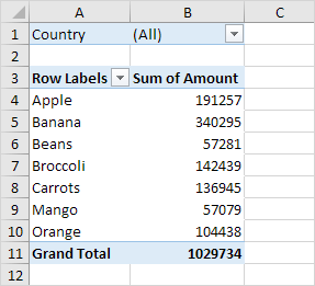
Multi-level Pivot Table - Easy Excel Tutorial First, insert a pivot table. Next, drag the following fields to the different areas. 1. Country field to the Rows area. 2. Amount field to the Values area (2x). Note: if you drag the Amount field to the Values area for the second time, Excel also populates the Columns area. Pivot table: 3. Next, click any cell inside the Sum of Amount2 column. 4. How to Customize Your Excel Pivot Chart Data Labels - dummies The Data Labels command on the Design tab's Add Chart Element menu in Excel allows you to label data markers with values from your pivot table. When you click the command button, Excel displays a menu with commands corresponding to locations for the data labels: None, Center, Left, Right, Above, and Below. None signifies that no data labels ... excel - Custom row labels in PivotTable - Stack Overflow 1. you can give nicknames to the fields that you are checking which populate the pivot table. If you go the pivot table data and right click you can change the value field settings to give a custom name to a row/series but I do not know about individual data points. path: pivot table data => right click => select Field Settings => edit custom name. How to Group Rows in Excel Pivot Table (3 Ways) - ExcelDemy Follow the steps below to create a PivotTable and then group the rows of dates in the table. 📌 Steps First, select anywhere in the dataset. Then, select the PivotTable icon from the Insert tab as shown in the following picture. Next, select the location for your PivotTable and then hit OK.

How to count unique values in pivot table?

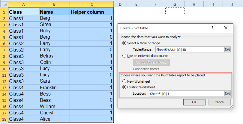
Automatic Row And Column Pivot Table Labels - How To Excel At Excel Select the data set you want to use for your table The first thing to do is put your cursor somewhere in your data list Select the Insert Tab Hit Pivot Table icon Next select Pivot Table option Select a table or range option Select to put your Table on a New Worksheet or on the current one, for this tutorial select the first option Click Ok

How to hide zero value rows in pivot table?

How to make row labels on same line in pivot table? Make row labels on same line with setting the layout form in pivot table As we all know, the pivot table has several layout form, the tabular form may help us to put the row labels next to each other. Please do as follows: 1. Click any cell in your pivot table, and the PivotTable Tools tab will be displayed. 2.

multiple fields as row labels on the same level in pivot table Excel - Microsoft Community

Excel Pivot Table Row labels - Stack Overflow Right click on the pivot, go to PivotTable Options, Display Tab. Click on "Classic Pivot Table Layout" Go to each field (column), right click, field settings, layout & print tab. Click on "Repeat Item Labels" That should give you the table you're looking for. Share Improve this answer answered Nov 9, 2015 at 13:20 user1923975 1,359 4 13 28

Solved: Convert excel matrix table to flattened table - Microsoft Power BI Community

Pivot Table adding "2" to value in answer set 1) Right click your pivot table -> Pivot table options -> Data -> Change "Number of items to retain per field" to NONE 2) Wipe all rows in your data source except for the headers 3) Refresh the pivot table 4) Save, and close all instances of Excel 5) Reopen the file, and paste your data 6) Refresh the pivot table

Pivot Tables - Easy Excel Tutorial

Design the layout and format of a PivotTable Click anywhere in the PivotTable. This displays the PivotTable Tools tab on the ribbon. On the Options tab, in the PivotTable group, click Options. In the PivotTable Options dialog box, click the Layout & Format tab, and then under Layout, select or clear the Merge and center cells with labels check box.

How to Sort Pivot Table Row Labels, Column Field Labels and Data Values with Excel VBA Macro ...

How to add side by side rows in excel pivot table - AnswerTabs To display more pivot table rows side by side, you need to turn on the Classic PivotTable layout and modify Field settings. For example will be used the following table: You have to right-click on pivot table and choose the PivotTable options. Then swich to Display tab and turn on Classic PivotTable layout:

Share :