45 pie chart excel labels

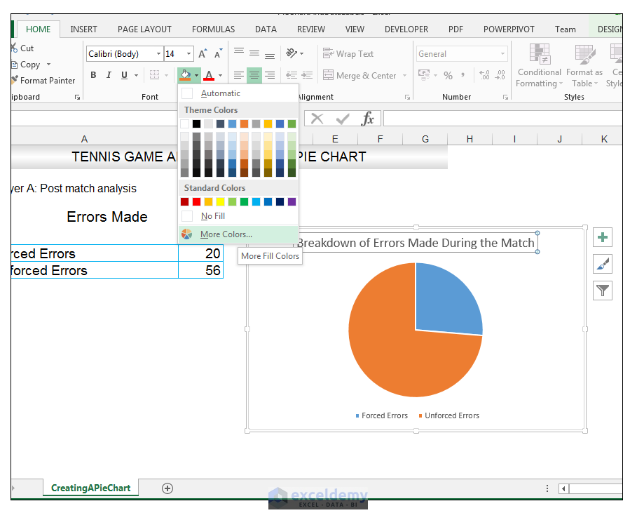
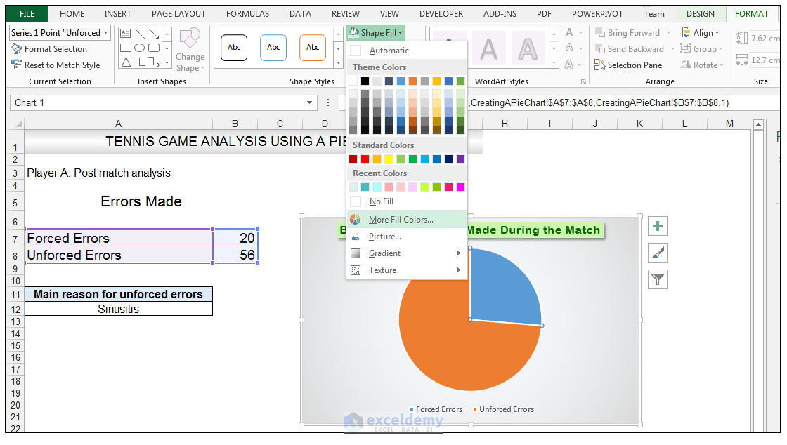
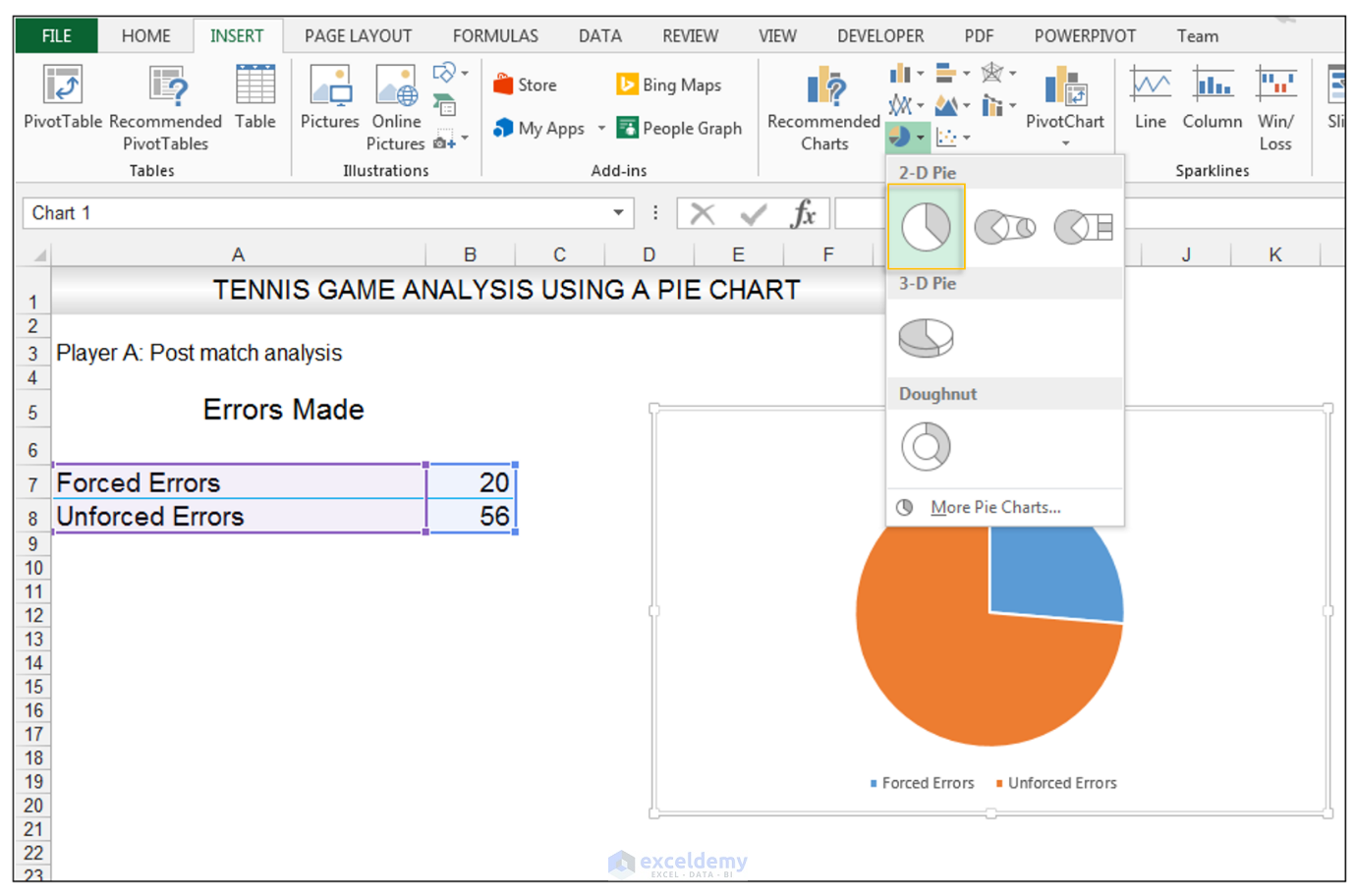
How to Make a Pie Chart in Excel & Add Rich Data Labels to The Chart! Creating and formatting the Pie Chart 1) Select the data. 2) Go to Insert> Charts> click on the drop-down arrow next to Pie Chart and under 2-D Pie, select the Pie Chart, shown below. 3) Chang the chart title to Breakdown of Errors Made During the Match, by clicking on it and typing the new title. Excel custom pie chart labels - Microsoft Community Excel custom pie chart labels. I want to use a pivot table to make a pie chart out of this. I want each of the pieces of the pie to contain the number of entries and between parentheses the percentage. So in the "Yes" piece, there should be '3 (33%)'. Actually, if I hover the pie chart in Excel, I get exactly the notation O want!

How to Create and Format a Pie Chart in Excel - Lifewire Select the plot area of the pie chart. Right-click the chart. Select Add Data Labels . Select Add Data Labels. In this example, the sales for each cookie is added to the slices of the pie chart. Change Colors When a chart is created in Excel, or whenever an existing chart is selected, two additional tabs are added to the ribbon.

Pie chart excel labels

Excel pie chart labels overlap arizona golden gloves. Search: R Pie Chart Labels Overlap.For example, x=[0,0 Click the Design tab in the Chart Tools section of the ribbon Instead of an overlapping window, graphics created in RStudio display inside the Plots pane A bar chart is a chart that visualizes data as a set of rectangular bars, their lengths being proportional to the values they represent To create a Bar of Pie chart ... excel - Positioning data labels in pie chart - Stack Overflow Positioning data labels in pie chart. I'm trying to format some charts I have, using VBA. To get started I recorded a macro of me doing what I wanted, to have an idea of what methods I'd want etc. The recorded macro looks like this - I'm including the whole thing, though the line to pay attention to is Selection.Position = xlLabelPositionCenter. Chart Legend / Data Labels In Pie Chart | MrExcel Message Board Add the data labels. Then, right click on any data label to select all the data labels for that series and select Format Data Labels... From the Label Options tab, in the Label Contains section, select the 'Series Name' checkbox. The above applies to Excel 2007. Excel 2003 supports the same capability though the dialog box choices may be different.

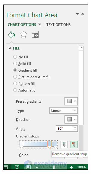
Pie chart excel labels. Edit titles or data labels in a chart - support.microsoft.com On a chart, click the label that you want to link to a corresponding worksheet cell. On the worksheet, click in the formula bar, and then type an equal sign (=). Select the worksheet cell that contains the data or text that you want to display in your chart. You can also type the reference to the worksheet cell in the formula bar. Create a Pie Chart in Excel (In Easy Steps) Select the pie chart. 9. Click the + button on the right side of the chart and click the check box next to Data Labels. 10. Click the paintbrush icon on the right side of the chart and change the color scheme of the pie chart. Result: 11. Right click the pie chart and click Format Data Labels. 12. How to Create a Bar of Pie Chart in Excel (With Example) Step 3: Customize the Bar of Pie Chart. By default, Excel has chosen to group the four smallest slices in the pie into one slice and then explode that slice into a bar chart. To group together a different number of slices, simply double click any element in the bar chart. This will bring up a panel called Format Data Series. We can also choose ... Add Labels with Lines in an Excel Pie Chart (with Easy Steps) To enables the data labels on the pie chart, Click on the Pie Chart first. Then click on the plus icon at the top-right corner of the pie chart. Now select Data Labels in the Chart Elements list. After that, you will see a variety of data labels position option such as, Center Inside End Outside End Best Fit Data callout

Pie of Pie Chart in Excel - Inserting, Customizing, Formatting Inserting a Pie of Pie Chart. Let us say we have the sales of different items of a bakery. Below is the data:-. To insert a Pie of Pie chart:-. Select the data range A1:B7. Enter in the Insert Tab. Select the Pie button, in the charts group. Select Pie of Pie chart in the 2D chart section. How to Create a Pie Chart in Excel | Smartsheet To create a pie chart in Excel 2016, add your data set to a worksheet and highlight it. Then click the Insert tab, and click the dropdown menu next to the image of a pie chart. Select the chart type you want to use and the chosen chart will appear on the worksheet with the data you selected. Is there a way to change the order of Data Labels? Replied on April 4, 2018. Hi Keith, I got your meaning. Please try to double click the the part of the label value, and choose the one you want to show to change the order. Thanks, Rena. -----------------------. * Beware of scammers posting fake support numbers here. * Once complete conversation about this topic, kindly Mark and Vote any ... How to Create a Pie Chart in Microsoft Excel And, by utilizing basic tools in Microsoft Excel, a pie chart is extremely simple to create. Step 1: Add Data in the Spreadsheet. ... You first need to select the plot section of the pie chart to add data labels to it. After that, right-click on the chart and click on the Add Data Labels option. Then, choose Add Data Labels once more from the ...

How to Show Pie Chart Data Labels in Percentage in Excel Click anywhere on the Pie Chart, and the Chart Elements icon will appear on the right side. Next, click on it and then click on the right arrow icon beside the Data Labels option. Later, select More Options from the appeared menu. Soon after, you will get the Format Data Labels field on the right side of your sheet. Add or remove data labels in a chart - support.microsoft.com Click the data series or chart. To label one data point, after clicking the series, click that data point. In the upper right corner, next to the chart, click Add Chart Element > Data Labels. To change the location, click the arrow, and choose an option. If you want to show your data label inside a text bubble shape, click Data Callout. Excel Pie Chart Labels on Slices: Add, Show & Modify Factors First of all, double-click on the data labels on the pie chart. As a result, a side window called Format Data Labels will appear. Then, go to the drop-down of the Label Options to Label Options tab. After that, check the Percentages option and uncheck all other options. You will get the percentages in the data labels. Pie Chart in Excel - Inserting, Formatting, Filters, Data Labels Right click on the Data Labels on the chart. Click on Format Data Labels option. Consequently, this will open up the Format Data Labels pane on the right of the excel worksheet. Mark the Category Name, Percentage and Legend Key. Also mark the labels position at Outside End. This is how the chark looks. Formatting the Chart Background, Chart Styles

Pie Chart - PK: An Excel Expert

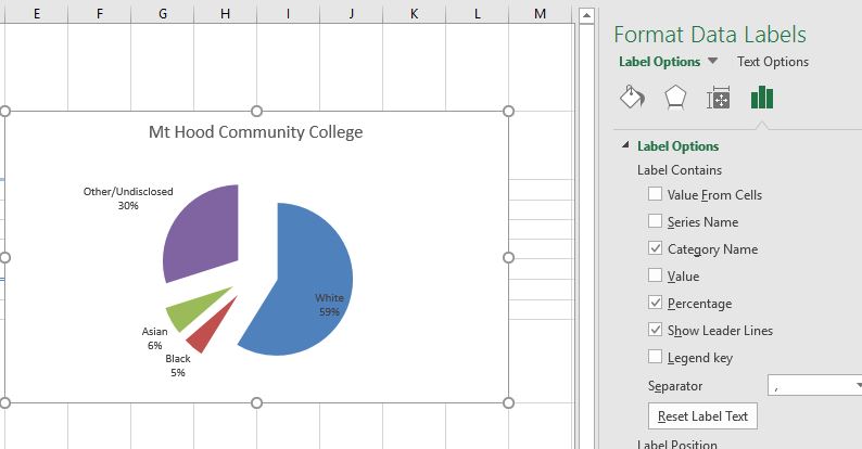
How to display leader lines in pie chart in Excel? - ExtendOffice To display leader lines in pie chart, you just need to check an option then drag the labels out. 1. Click at the chart, and right click to select Format Data Labels from context menu. 2. In the popping Format Data Labels dialog/pane, check Show Leader Lines in the Label Options section. See screenshot: 3.

31 Label Pie Chart Excel - Labels For You

Move data labels - support.microsoft.com Right-click the selection > Chart Elements > Data Labels arrow, and select the placement option you want. Different options are available for different chart types. For example, you can place data labels outside of the data points in a pie chart but not in a column chart.

How to Make a Pie Chart in Excel & Add Rich Data Labels to The Chart!

Multiple data labels (in separate locations on chart) Running Excel 2010 2D pie chart I currently have a pie chart that has one data label already set. The Pie chart has the name of the category and value as data labels on the outside of the graph. I now need to add the percentage of the section on the INSIDE of the graph, centered within the pie section. I'm aware that I could type in the percentages as text boxes, but I want this graph to ...

How to Make a Pie Chart in Excel & Add Rich Data Labels to The Chart!

Add a pie chart - support.microsoft.com Click Insert > Insert Pie or Doughnut Chart, and then pick the chart you want. Click the chart and then click the icons next to the chart to add finishing touches: To show, hide, or format things like axis titles or data labels, click Chart Elements . To quickly change the color or style of the chart, use the Chart Styles .

Excel: How to make an Excel-lent bull's-eye chart

pie chart - Hide a range of data labels in 'pie of pie' in Excel ... Next select any slice from the main chart and hit CTRL+1 to bring up the Series Option window, here set the gap width to 0% (this will centre the main pie as much as possible) and set the second plot size to 5% (which is the minimum it will allow), and you have made your second pie invisible! Share answered Sep 7, 2015 at 1:02 Nobody 1

How to Create a Pie Chart in Excel | Smartsheet

excel - How to not display labels in pie chart that are 0% - Stack Overflow Generate a new column with the following formula: =IF (B2=0,"",A2) Then right click on the labels and choose "Format Data Labels". Check "Value From Cells", choosing the column with the formula and percentage of the Label Options. Under Label Options -> Number -> Category, choose "Custom". Under Format Code, enter the following:

How to insert data labels to a Pie chart in Excel 2013 - YouTube

Formatting data labels and printing pie charts on Excel for Mac 2019 ... Here's a work around I found for printing pie charts. Still can't find a solution for formatting the data labels. 1. When printing a pie chart from Excel for mac 2019, MS instructions are to select the chart only, on the worksheet > file > print. Excel is supposed to print the chart only (not the data ) and automatically fit it onto one page.

How to Create and Label a Pie Chart in Excel 2013 : 8 Steps - Instructables

Change the format of data labels in a chart To get there, after adding your data labels, select the data label to format, and then click Chart Elements > Data Labels > More Options. To go to the appropriate area, click one of the four icons ( Fill & Line, Effects, Size & Properties ( Layout & Properties in Outlook or Word), or Label Options) shown here.

SQL & BI Learning: Pie Chart with data labels outside in ssrs

Pie Chart in Excel | How to Create Pie Chart - EDUCBA Pie Chart in Excel is used for showing the completion or main contribution of different segments out of 100%. It is like each value represents the portion of the Slice from the total complete Pie. For Example, we have 4 values A, B, C and D.

Excel Chapter 2 – Business Computers 365

How to Edit Pie Chart in Excel (All Possible Modifications) How to Edit Pie Chart in Excel 1. Change Chart Color 2. Change Background Color 3. Change Font of Pie Chart 4. Change Chart Border 5. Resize Pie Chart 6. Change Chart Title Position 7. Change Data Labels Position 8. Show Percentage on Data Labels 9. Change Pie Chart's Legend Position 10. Edit Pie Chart Using Switch Row/Column Button 11.

How to Make a Pie Chart - ExcelNotes

Chart Legend / Data Labels In Pie Chart | MrExcel Message Board Add the data labels. Then, right click on any data label to select all the data labels for that series and select Format Data Labels... From the Label Options tab, in the Label Contains section, select the 'Series Name' checkbox. The above applies to Excel 2007. Excel 2003 supports the same capability though the dialog box choices may be different.

Quickly create a half pie chart in Excel

excel - Positioning data labels in pie chart - Stack Overflow Positioning data labels in pie chart. I'm trying to format some charts I have, using VBA. To get started I recorded a macro of me doing what I wanted, to have an idea of what methods I'd want etc. The recorded macro looks like this - I'm including the whole thing, though the line to pay attention to is Selection.Position = xlLabelPositionCenter.